Introduction

When I first started learning algorithms and data structures, every resource I came across would mention Dijkstra’s algorithm in a sort of mystical, this-is-beyond-your-lowly-understanding manner. I disagree with that approach (in fact, I disagree with that approach for just about everything). Now that I’ve actually invested some time into learning it, it really isn’t as frightful as I was told to believe. I will (to the best of my ability) elucidate Dijkstra’s algorithm here.

Single source shortest path

Dijkstra’s algorithm is used to solve the single source shortest path. What does that mean? Starting at a single point, what is the shortest path to another point, say X. The best example would be using Google maps to get from your location to a destination. Using an algorithm (not necessarily Dijkstra’s) we can compute the shortest path by space and/or time. Let’s say you are given the diagram below, each node depicts a certain location and the number in blue a “distance” between to the two node. What is the shortest path from node S to H?

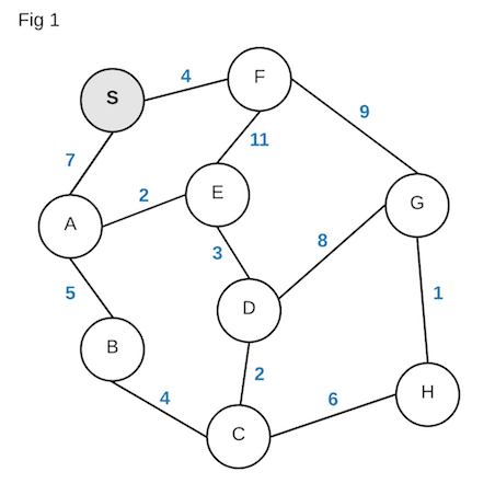
It is not so obvious at first glance. Indeed, this is also only a simple example. Imagine the entirety of Manhattan mapped out. The complexity of the diagram would increase by a million-fold! Having said that, we will come back to this diagram to solve our problem. For now we require some additional background knowledge before we go about implementing Dijkstra’s algorithm.

Breadth-first search

At its heart, Dijkstra’s algorithm is really only a modified breadth-first search. Breadth-first search (BFS) is a graph traversal algorithm which works by exploring all neighboring nodes first, before moving on to the next level of neighbors (neighbors’ neighbors). Let’s see how this would play out using the figure above (forgetting about the numbers for a minute) starting at S:

We see that S has 2 neighbors, A and F. We add these on our todo list to explore (marked in gray). We start with A which was at the top of our todo list. A likewise has 2 neighbors, E and B – so we add those to our todo list. We’ve now fully explored A (black) so we move on to the next item on our todo list, F. We explore F and see that it has two neighbors as well, E and G. We again add those two to our todo list. We are now done exploring F and see that the top of our list has E, so we start exploring that. Lucky for us, E only has one neighbor we have yet to explore, and that is D.

I won’t belabor you by writing out every step, but you can see the pattern here: we explore a node, add its neighbors to our todo list, explore those neighbors. A caveat that I should mention is that we never explore the same node twice. In our diagram above, both A and F have E as their neighbor. When we explore E we make sure to mark it as explored so that we don’t explore it again. Eventually, we’ll have explored all the nodes! But where is the logic coming from for this magical “todo list”? That is our next topic…

The queue

I hand-waved our addition of the nodes to a todo list, but it is a legitimate data structure with a name: a queue. Breadth-first search uses a queue to keep track of nodes not yet explored. A queue is a first-in-first-out (FIFO) data structure. This means that the first item to be added, will be the first item to be removed. Think of a queue as a waiting line at a grocery store checkout station. There might be people ahead of you, in which case you will have to wait your turn until all the ones who came before you have been checked out. The queue’s most important operations are enqueue which adds an item to the end, and dequeue which removes the first item in line.

A simple BFS implementation

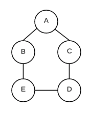
Now that we know about a queue, let’s build a simple implementation of breadth-first search. I won’t get into the specifics of graph representation in code, but it is typically represented as an “adjacency list” – a hash object with the keys as nodes, and the values as neighbors:

# Simple graph representation like adjacency list
# using an array to represent our list
graph = {
  'A': ['B', 'C'],
  'B': ['A', 'E'],
  'C': ['A', 'D'],
  'D': ['C', 'E'],
  'E': ['B', 'D']
}

And this is how this graph would look like:

Now let’s implement BFS:

def bfs(graph, source)
  q = Queue.new
  # Keep track of what we've explored
  explored = Hash.new

  # Start at source node
  q.enqueue(source)

  # While our queue is not empty,
  # keep going through nodes
  while !q.empty?
    node = q.dequeue
    explored[node] = true
    # Get the neighbor nodes
    neighbors = graph[node]

    # For each neighbor node, add it to the queue
    # unless we've previously explored it
    neighbors.each do |v|
      q.enqueue(v) unless explored[v]
    end
  end
end

This will traverse our graph layer-by-layer, node-by-node. This is as barebones as it gets of course but it gives us an idea of how a BFS algorithm would look like and how we can modify it to fit our needs.

Enter the priority queue

One of Dijkstra’s algorithm modifications on breadth-first search is its use of a priority queue instead of a normal queue. With a priority queue, each task added to the queue has a “priority” and will slot in accordingly into the queue based on its priority level.

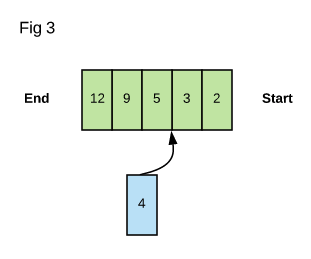
The figure above shows a queue consisting of items with rankings based on priority. In this case, the item with priority 2 would be dequeued next. If we were to enqueue the blue item with priority 4 next, it would go before the item with priority 5 but after the one ranked 3. This is known as a minimum priority queue – the smallest priority will be highest ranked and will be processed first.

Implementing Dijkstra’s algorithm

We’ve now been introduced to all of the pieces of the puzzle – let’s fit them together. We will use the priority queue in place of the normal queue in our modified BFS – with the priorities being the distances between nodes. How will this work out? Let’s go step by step:

1. Initialize source node with a distance of 0 since we are starting here
2. Initialize all other nodes with an infinite distance
3. Start the queue loop after inserting our source node into it
4. For each neighbor of our node, calculate the tentative distance between the current node’s distance and the distance to its neighbor
   • If the tentative distance is less than the distance of the neighbor, set that neighbor node’s distance to the tentative distance and enqueue it with that distance as its priority
     (This is known as Dijkstra’s greedy score)
5. Continue through the priority queue until we’ve calculated all nodes' shortest path to source
   • Optionally, we can provide a target node and as soon as that node is dequeued, we can stop our search

Let’s see these steps in action using the graph we started with:

Based on the animation above, our shortest path from S to H is S->F->G->H and has a distance of 14. Another thing to note is that our algorithm calculated the shortest distance for every node from the source. The animation above “dropped” paths that did not satisfy Dijkstra’s greedy score. In actuality the algorithm will just not enqueue any node that does not satisfy the greedy score.

Let’s see the algorithm implementation:

def dijkstra(graph, source)
  pq = PriorityQueue.new
  # Initialize distances for all nodes at infinity
  dist = Hash.new(Float::INFINITY)
  # Get edge lengths
  lengths = graph.get_lengths

  # Initialize source node and insert into queue
  dist[source] = 0
  # Priority queue holds nodes as key/value pairs
  pq.enqueue(source, dist[source])

  while !pq.empty?
    node = pq.dequeue[:key]
    neighbors = graph[node]

    neighbors.each do |neighbor|
      # Calculate tentative distance 
      # (Dijkstra's greedy score)
      tent_dist = dist[node] + lengths[node][neighbor]
      
      if tent_dist < dist[neighbor]
        # Set neighbor's new distance as it is shorter
        dist[neighbor] = tent_dist
        # Enqueue using new distance as priority
        pq.enqueue(neighbor, dist[neighbor])
      end
    end
  end
  return dist # Or whatever else you want
end

This algorithm looks very similar to BFS! We just added the calculation of the greedy score which determined how to prioritize insertion into our priority queue. One thing to note is I glanced over getting edge lengths as it is just a detail of implementation. The usual way to do this is to construct a 2-dimensional matrix between nodes and fill out lengths. It can also be done by creating a hash.

Improvements and other thoughts

As it stands, the running time of our algorithm is not too great. If we assume a naive implementation of a priority queue (enqueue will scan entire structure to find place to insert), then our algorithm is running in quadratic time O(mn).

Can we do better? Of course! We can implement our priority queue using a heap. A heap will provide the same API to us as a priority queue (enqueue/insert, dequeue/extract) but it does insertion in logarithmic time. That’s great news! That means we effectively go from O(mn) to O(m log n) time by using a heap.

The implementation above does not map out the paths. The algorithm can easily be augmented to accomodate that by creating a predecessor hash which can be added to as we are enqueue-ing. We can also stop the algorithm earlier if we provide to it a target node: as we are dequeue-ing, we can just check if that is the node we are looking for. If so, we return from the algorithm with the distance to that node. Our current implementation goes through every node.

A caveat I forgot to mention earlier is that this algorithm requires positive edge lengths and will break with negative edge lengths. There is Bellman-Ford algorithm for that situation.

Fin

This has been a fun dive into a famous algorithm. It is elegant, and surprisingly simple once we spent a little time into it. I hope you enjoyed reading this as much as I enjoyed creating it!