| tags: [ algorithms ]
Computing Strongly Connected Components
Introduction
I am currently working through Stanford’s algorithms course as part of “learning my fundamentals”, and one difficult and interesting topic that I’ve encountered is computing strongly connected components of a directed acyclic graph.
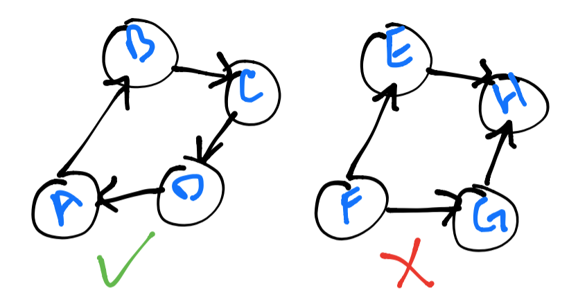
A graph is said to be strongly connected if every vertex is reachable from
every other vertex. In the image below, you will notice that the left graph
is strongly connected, but the right one is not – vertex H acts as a sink
for every vertex with a connection and it is not possible to reach any other vertex
from here.

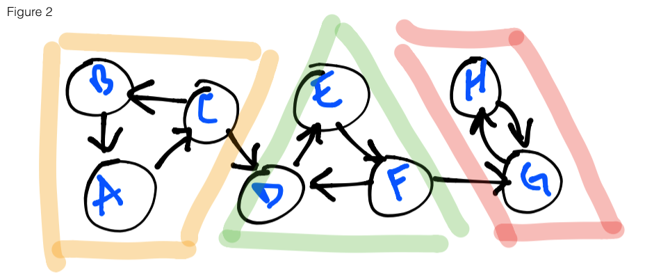
A graph can also contain multiple strongly connected components, each being a strongly connected subgraph.
In the figure 2 below, three strongly connected components (henceforth will be
known by the abbreviation: SCCs) are highlighted: yellow, green and red. If a
graph is entered at any vertex using depth-first search (DFS) as our traversal algorithm,
it is possible to reach any of the vertices that are highlighted with the same
color. For example, entering the graph at the vertex E, I am able to reach F
and D. Likewise for vertex B with A and C, etc. You’ll also notice that
there are some vertices that, upon exploration, can also lead to other components
– this will be the crux of our problem today.

The problem
In figure 2 above, you’ll notice that if we start at vertex B, we are able to
correctly explore all of the orange SCC. The problem arises when we start at A
or C. There is a possibility that when we reach C the next vertex explored
will be D and not B. If this occurs, we will incorrectly miss identifying the
orange SCC. How then can we solve this problem? The astute observer will notice
that for the red SCC, exploring any point will correctly identify the SCC. This
is because there are no outbound edges – any point we hit will only explore the
two vertices and that’s it. This is the fundamental understanding required to
arrive at the solution.
Kosaraju’s two-pass algorithm
Kosaraju’s algorithm is a linear time algorithm to find strongly connected components. Our fundamental understanding will help us navigate this algorithm towards a solution. The algorithm solves this problem by going through the graph twice (using DFS): first through the transposed version of the graph (reversed), second through normally.
Why reversed? The first pass will collect the finishing times for all the vertices and compute a magical ordering. The second pass will go through the vertices in descending order of finishing times and compute the leaders.
The solution
To recap, the algorithm is composed of two parts:
- Loop through all vertices in the transposed graph – running DFS on each if it has not been explored and collecting the finishing time of each vertex
- Loop through all the vertices in the normal graph in descending order of finishing times – running DFS on each if it has not been explored and collecting the leader nodes

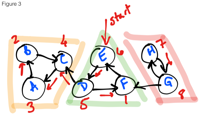
Figure 3 shows the first step of the algorithm. Starting at E, we loop through
the vertices on the reverse graph, running DFS on each vertex (if it has not been
explored) and collecting the finishing times (denoted in red).

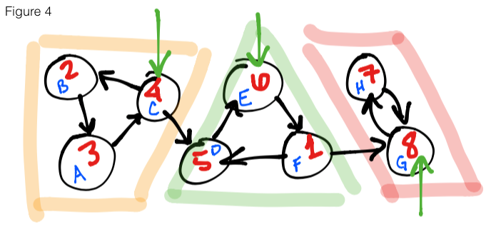
Figure 4 shows the second step of the algorithm. We substitue the vertex names
for their finishing times, un-reverse the edges, then start a DFS on the highest
finishing time moving in descending order. In the figure, we start at 8 – marking
it as leader node – then continue on to 7 and end this run because all reachable
vertices have been explored. We move on to the next highest finishing time, 6,
marking it as leader and explore all adjacent vertices. Once we are finished with
this SCC, we see that the next unexplored vertex is 4, so we start there, mark it
as leader and explore the final 2 vertices. As you might notice, the leaders we
have collected are { 8, 6, 4 } (green arrows), and that is exactly the amount
of SCCs in this graph.
Final thoughts
This was an interesting and difficult algorithm and has definitely given me confidence in working with graph-based problems. I wrote it in JavaScript using Node as my run-time environment for execution. It worked well enough for small datasets (using an adjacency list as my graph representation) but when I encountered larger datasets I ran into a lot of issues with stack and heap overflows as my implementation of DFS was recursive (I was also creating the reverse graph and storing it in memory). Even after optimizations (using a stack to store finishing times, using a hash table of sets for my adjancency list), I ended up needing to increase the maximum stack size as well as the heap size. These options can be found under V8 options. Ultimately, my run command became:
$ node --max-old-space-size=4096 --stack-size=10000 sccs.js
- Heap size:
--max-old-space-size - Stack size:
--stack-size
I was able to get a solution in under 5 seconds with a dataset of 70mb. Once again, I owe all this to Stanford’s algorithm course and particularly the professor, Tim Roughgarden. He is an excellent teacher and I highly recommend the course.